Aim

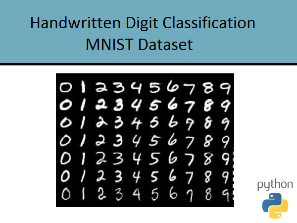
We have a data set of handwritten digits (MNIST) and our aim is to build a classifier to identify which digit the image represents. In technical terms, we have to design a classifier with 10 classes representing the digit. We will use three strategies to solve the same problem:

1. Bayes Classifier: Ipython Notebook
2. Gradient Descent using softmax function
3. Feed forward Neural Network using backpropagation learning

Data:

Data was obtained from the following website:

http://yann.lecun.com/exdb/mnist/index.html

Each digit is represented as a 28x28 dimensional image or 784 pixels. Each image is in grayscale format. Hence a typical “feature vector” we will draw out from this image will be 784-dimensional

Strategy 1: Using Multivariate Bayes Classification

We will perform handwritten digit classification designing a Bayes Optimal classifier using a Gaussian generative model on MNIST Dataset. We will model each class(representing each digit as a multivariate (784-dimensional) Gaussian. The data set of handwritten digits was obtained from: This is called generative parametric modeling as we model the classes and NOT the class boundaries.

Steps

1. We will load the set of training and testing dataset images. We will be defining a function for that.
2. Then we will split the dataset into 2 parts - 1 for training and other for validation.
3. Then we will fit a Bayesian generative model on training dataset. This involves two steps: a. Determine class probabilities (easier task) b. Fit a Gaussian for each digit and find its mean and covariance (likelihood) (harder task)
4. Now we can use Bayes Rule for classification (Maximize Posterior Probability)
5. Find the validation error

Visualization

In order to gain more insights as to how the Bayesian classifier works we could do two visualizations.

• Since we know the true class of each digit, we could plot a histogram to get the absolute number of misclassifications over actual digits.
• We could also plot a heatmap where one axis comprise of actual digit and the other comprises of the predicted digit. Both visualizations are provided in the Ipython notebook (link given above)

The latter plot will sort of show interesting insights: The classifier predicts a lot of “5”’s and “3”’s as “8”’s. One thing we could infer from this analysis is maybe the lower half loop in 3 and 5, might be perceived as a lower half loop in “9”. It was also observed that as a lot of people do not write the lower half loop of “9”, A lot of cases when the true class was “1” or “7” was often predicted as a “9”. The max misclassifications occur for the digits “5”, followed by a few for “7”. This Bayes Classifier had an error value 0.16 (85% accuracy) on the test set. This was implemented in Python.

Strategy 2: Stochastic Gradient Descent

We define the softmax function as follows: $y_{pred} = max_i [\frac{e^{w_i^TX}}{\sum_j(e^{w_j^TX})})$ We will use iterative gradient descent to solve for the weight matrices

Steps

Initialization Steps

1. We will load the set of training and testing dataset images. We will be using same function as above.
2. Then we will split the dataset into 2 parts - 1 for training and other for validation.
3. We will use the softmax function to predict probabilities of each class. We initial the weight matrices w_i for each class.
4. In order to control our gradient descent and avoid divergence, we introduce an annealing step. We introduce a learning parameter \eta and initialize it to some small value. (Note that the choice of eta controls the speed of descent. Aim is to choose an optimal eta that mages convergence fastest)
5. In order to avoid overfitting, we will use regularization. Now we could use 2 kinds of regularization L-1 and L-2. We will explore for both kinds of regularation. This will lead to another regularization parameter (\lambda)
6. We now define the loop

Loop

• Based on current weights predict training labels
• Find training error gradient.
• Add regularization term to error gradient (For L1: lambda*sign(w); For L2: 2 (lambda *w))
• Update weight matrix: w = w - eta * gradient
• Find validation set loss, test set loss and accuracies
• Define break condition (iterations > 1000) then break

This is a sophisticated approach which gives us the luxury to tune clasifier for optimal hyperparameters. Depending upon the accuracy we need we can change the break condition.

However like most gradient descent algorithms, it takes ages to reach high levels of accuracy. The initial learning curve is high and reaches 70-75% in a few iterations. However every successive percent increase takes more number of epochs. I was able to achieve around 80% in 1000 epochs. This SGD algorithm was implemented in MATLAB.

Strategy 3: Neural Network

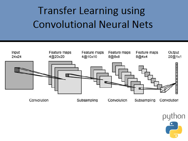
Here we basically train a feedforward neural network using Backpropagation to determine the weights to predict the classes for the given input. Since input is of 784 length, our input layer will have 784 nodes. Output layer will have 10 nodes (representing each class). We will then create a densely connected feed forward neural net between these two layers. We have the luxury to choose the intermediate hidden architecture. We can vary number of hidden layers/ number of nodes in each layer etc.

Results: Achieved a test accuracy of 96.08%

Project Details

Date: May 25, 2014

Categories: project

Tags: Python, Bayesian Inference, Stochastic GD, Batch learning, Neural Network, Backprop

Website: